38 excel pie chart with lines to labels
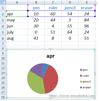
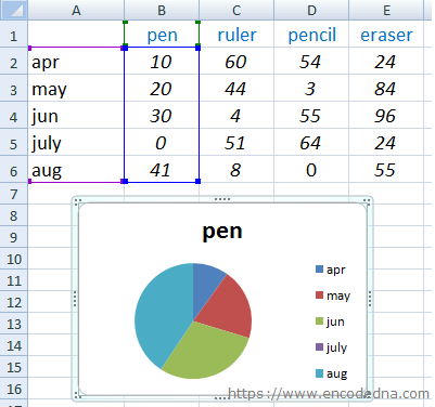
Create a Pie Chart in Excel (In Easy Steps) 1. Select the range A1:D2. 2. On the Insert tab, in the Charts group, click the Pie symbol. 3. Click Pie. Result: 4. Click on the pie to select the whole pie. Click on a slice to drag it away from the center. Result: Note: only if you have numeric labels, empty cell A1 before you create the pie chart. Excel Doughnut chart with leader lines - teylyn Select the pie chart and add data labels. They will be positioned outside of the pie. Click each data label and drag it a bit to see the leader lines appear. Step 3 - Add data labels for the pie chart Step 4 - Hide the pie chart. Now that the data labels and the leader lines are in place, we can hide the pie chart.
Create a Line Chart in Excel (In Easy Steps) - Excel Easy After creating the chart, you can enter the text Year into cell A1 if you like. Let's customize this line chart. To change the data range included in the chart, execute the following steps. 4. Select the line chart. 5. On the Chart Design tab, in the Data group, click Select Data. 6. Uncheck Dolphins and Whales and click OK. Result:
Excel pie chart with lines to labels
How to add leader lines to doughnut chart in Excel? Select data and click Insert > Other Charts > Doughnut. In Excel 2013, click Insert > Insert Pie or Doughnut Chart > Doughnut. 2. Select your original data again, and copy it by pressing Ctrl + C simultaneously, and then click at the inserted doughnut chart, then go to click Home > Paste > Paste Special. See screenshot: 3. Pie Chart in Excel | How to Create Pie Chart - EDUCBA Step 1: Select the data to go to Insert, click on PIE, and select 3-D pie chart. Step 2: Now, it instantly creates the 3-D pie chart for you. Step 3: Right-click on the pie and select Add Data Labels. This will add all the values we are showing on the slices of the pie. How to Create Pie of Pie Chart in Excel? - GeeksforGeeks Creating Pie of Pie Chart in Excel: Follow the below steps to create a Pie of Pie chart: 1. In Excel, Click on the Insert tab. 2. Click on the drop-down menu of the pie chart from the list of the charts. 3. Now, select Pie of Pie from that list. Below is the Sales Data were taken as reference for creating Pie of Pie Chart:
Excel pie chart with lines to labels. Formatting data labels and printing pie charts on Excel for Mac 2019 ... Work around: Select the area of the chart - by selecting the cells behind where the chart is sitting > Print area> Select print area>File > print>then set print perameters (paper size, fit to page etc.) > Print. This worked. 2. When formatting data labels on an extended bar of pie chart: Excel does not allow me to: Pie of Pie Chart in Excel - Inserting, Customizing, Formatting Inserting a Pie of Pie Chart. Let us say we have the sales of different items of a bakery. Below is the data:-. To insert a Pie of Pie chart:-. Select the data range A1:B7. Enter in the Insert Tab. Select the Pie button, in the charts group. Select Pie of Pie chart in the 2D chart section. Leader Lines in Excel Pie Charts - Microsoft Community I've created pie charts in Excel. When I move the labels around I get leader lines that I do not want. I can delete them but if I save, close and then open the file, they come back. I can format the lines so that the color is white and they do not show. But again, if I save, close and reopen, the lines turn back to black. Pie Chart in Excel - Inserting, Formatting, Filters, Data Labels To insert a Pie Chart, follow these steps:- Select the range of cells A1:B7 Go to Insert tab. In the charts group, Select the pie chart button Click on pie chart in 2D chart section. Adding Data Labels The default pie chart inserted in the above section is:-
Display data point labels outside a pie chart in a paginated report ... Create a pie chart and display the data labels. Open the Properties pane. On the design surface, click on the pie itself to display the Category properties in the Properties pane. Expand the CustomAttributes node. A list of attributes for the pie chart is displayed. Set the PieLabelStyle property to Outside. Set the PieLineColor property to Black. Put labels inside pie chart - MrExcel Message Board Dec 2, 2003. #2. Select and Format the data labels using the Label Position setting on the Alignment tab. N. Directly Labeling in Excel - Evergreen Data There are two ways to do this. Way #1 Click on one line and you'll see how every data point shows up. If we add a label to every data points, our readers are going to mount a recall election. So carefully click again on just the last point on the right. Now right-click on that last point and select Add Data Label. THIS IS WHEN YOU BE CAREFUL. Prevent overlapping of data labels in pie chart - Stack Overflow You may be able to start with this answer - chris neilsen Apr 28, 2021 at 2:37 Add a comment 1 Answer Sorted by: 1 Did you try Best Fit option under Format Data Labels -> Label Options Image attached. Share Improve this answer answered Apr 28, 2021 at 2:28 Die-Bugger 163 7
How to Add Leader Lines in Excel? - GeeksforGeeks Step 1: Select a range of cells for which you want to make a line chart. Step 2: Go to Insert Tab and select Recommended Charts. A dialogue box name Insert Chart appears. Step 3: Click on All Charts and select Line. Click Ok. Step 4: A line chart is embedded in the worksheet. Step 5: Go to Chart Design Tab and select Add Chart Element . How-to Add Label Leader Lines to an Excel Pie Chart - YouTube Step-by-Step Tutorial: how-to create label leader lines that connect pie labels that are outsi... Add data labels and callouts to charts in Excel 365 - EasyTweaks.com Step #1: After generating the chart in Excel, right-click anywhere within the chart and select Add labels . Note that you can also select the very handy option of Adding data Callouts. Step #2: When you select the "Add Labels" option, all the different portions of the chart will automatically take on the corresponding values in the table ... Excel Pie Chart Labels on Slices: Add, Show & Modify Factors We have to follow the following steps to insert the pie chart with data labels. 📌 Steps: First, select the range of cells B5:C12. After that, in the Insert tab, click on the drop-down arrow of the Insert Pie or Doughnut Chart. Then, choose the 3-D Pie option from the 3-D Pie section. The chart will appear in front of you.
33 How To Label Pie Chart In Excel - Labels Database 2020
Advanced Excel - Leader Lines - tutorialspoint.com A Leader Line is a line that connects a data label and its associated data point. It is helpful when you have placed a data label away from a data point. In earlier versions of Excel, only the pie charts had this functionality. Now, all the chart types with data label have this feature. Add a Leader Line. Step 1 − Click on the data label.

how to label pie chart in excel - Labels 2021
How to Create and Format a Pie Chart in Excel - Lifewire To add data labels to a pie chart: Select the plot area of the pie chart. Right-click the chart. Select Add Data Labels . Select Add Data Labels. In this example, the sales for each cookie is added to the slices of the pie chart. Change Colors

How to Create and Label a Pie Chart in Excel 2013 : 8 Steps - Instructables
Adding 2nd Data Label Series to Bar of Pie Chart - Excel Help Forum If you use 2 sets of the same data in the chart you can create 2 pie/bar charts, with one appearing on the secondary axis. Make sure the settings for bar/pie formatting are the same. Add data labels to each series. Format one to show names the other values. Within the pie you may want to delete the name data labels. Attached Files
How to Make Pie Chart with Labels both Inside and Outside - ExcelNotes
Add or remove data labels in a chart - support.microsoft.com To label one data point, after clicking the series, click that data point. In the upper right corner, next to the chart, click Add Chart Element > Data Labels. To change the location, click the arrow, and choose an option. If you want to show your data label inside a text bubble shape, click Data Callout.
Terrible Chart Tuesday - Leader Lines - Excel Dashboard Templates
excel - Positioning data labels in pie chart - Stack Overflow Sub tester () Dim se As Series Set se = Totalt.ChartObjects ("Inosa gule").Chart.SeriesCollection ("Grøn pil") se.ApplyDataLabels With se.DataLabels .NumberFormat = "0,0 %" With .Format.Fill .ForeColor.RGB = RGB (255, 255, 255) .Transparency = 0.15 End With .Position = xlLabelPositionCenter End With End Sub

How to Create and Label a Pie Chart in Excel 2013 : 8 Steps - Instructables
Change the format of data labels in a chart To get there, after adding your data labels, select the data label to format, and then click Chart Elements > Data Labels > More Options. To go to the appropriate area, click one of the four icons ( Fill & Line, Effects, Size & Properties ( Layout & Properties in Outlook or Word), or Label Options) shown here.
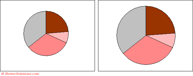
Excel Charts - Show Pie Charts in Proportion
Excel charts: add title, customize chart axis, legend and data labels Click anywhere within your Excel chart, then click the Chart Elements button and check the Axis Titles box. If you want to display the title only for one axis, either horizontal or vertical, click the arrow next to Axis Titles and clear one of the boxes: Click the axis title box on the chart, and type the text.

33 How To Label A Pie Chart In Excel - Labels 2021
Leader lines for Pie chart are appearing only when the data labels are ... I have a pie chart with data labels connected to leader lines. Though I have set the position of labels to 'Outside End', the leader lines are not appearing by default. It shows up only when I manually move the data labels. I dont have to move them far apart. Just a slight change in the position of labels helps.

How to Make a Pie Chart in Excel & Add Rich Data Labels to The Chart!
Add Labels with Lines in an Excel Pie Chart (with Easy Steps) Steps to Add Labels with Lines in an Excel Pie Chart Step-1: Insert a Pie Chart Step-2: Enable Data Labels Step-3: Add Labels with Lines Advantages of Using Pie Charts Disadvantages of Using Pie Charts Practice Section Conclusion Download Practice Workbook You can download the Excel file from the following link and practice along with it.
:max_bytes(150000):strip_icc()/Capture-5c84941446e0fb00013364fc.JPG)
33 How To Label Pie Chart In Excel - Labels Design Ideas 2020
Dynamically Label Excel Chart Series Lines - My Online Training Hub Select the outer edge of the chart to expose the contextual Chart Tools ribbon tabs Select the Format tab (In Excel 2007 & 2010 it's the Layout tab) Click on the drop down Select the first label series: Step 4: Add the Labels Excel 2013/2016 Click the + icon beside the chart as shown below (Note: for Excel 2007/2010 go to Layout tab) Data Labels
PIE chart labelling values with reference lines
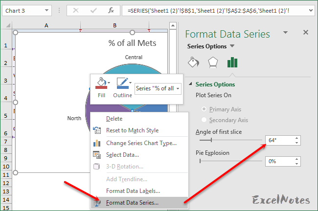
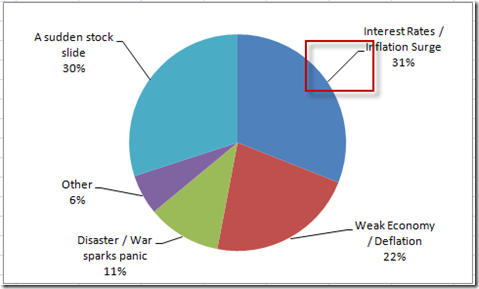
How to display leader lines in pie chart in Excel? To display leader lines in pie chart, you just need to check an option then drag the labels out. 1. Click at the chart, and right click to select Format Data Labels from context menu. 2. In the popping Format Data Labels dialog/pane, check Show Leader Lines in the Label Options section. See screenshot: 3.
33 How To Label A Pie Chart In Excel - Labels 2021
How to Create Pie of Pie Chart in Excel? - GeeksforGeeks Creating Pie of Pie Chart in Excel: Follow the below steps to create a Pie of Pie chart: 1. In Excel, Click on the Insert tab. 2. Click on the drop-down menu of the pie chart from the list of the charts. 3. Now, select Pie of Pie from that list. Below is the Sales Data were taken as reference for creating Pie of Pie Chart:
How-to Add Label Leader Lines to an Excel Pie Chart - Excel Dashboard Templates
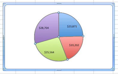
Pie Chart in Excel | How to Create Pie Chart - EDUCBA Step 1: Select the data to go to Insert, click on PIE, and select 3-D pie chart. Step 2: Now, it instantly creates the 3-D pie chart for you. Step 3: Right-click on the pie and select Add Data Labels. This will add all the values we are showing on the slices of the pie.
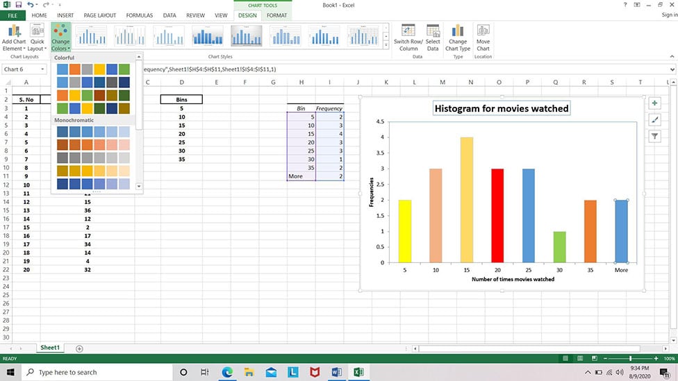
How to Create Histogram in Microsoft Excel? - My Chart Guide
How to add leader lines to doughnut chart in Excel? Select data and click Insert > Other Charts > Doughnut. In Excel 2013, click Insert > Insert Pie or Doughnut Chart > Doughnut. 2. Select your original data again, and copy it by pressing Ctrl + C simultaneously, and then click at the inserted doughnut chart, then go to click Home > Paste > Paste Special. See screenshot: 3.

Charts and Graphs Examples, Tutorials, and Samples for Microsoft Excel 2007
How to Create a Pie Chart in Excel | Smartsheet

How-to Add Label Leader Lines to an Excel Pie Chart - Excel Dashboard Templates

Excel 2013 Recommended Charts, Secondary Axis, Scatter & PivotCharts
Post a Comment for "38 excel pie chart with lines to labels"