42 remove data labels from excel chart
Excel Chart Data Labels - Microsoft Community Right-click a data point on your chart, from the context menu choose Format Data Labels ..., choose Label Options > Label Contains Value from Cells > Select Range. In the Data Label Range dialog box, verify that the range includes all 26 cells. When I paste your data into a worksheet, the XY Scatter data is in A2:B27, and the data labels are in ... How to Add and Remove Chart Elements in Excel Select the data, go to insert menu --> Charts --> Line Chart. 1: Add Data Label Element to The Chart. To add the data labels to the chart, click on the plus sign and click on the data labels. This will ad the data labels on the top of each point. If you want to show data labels on the left, right, center, below, etc. click on the arrow sign.
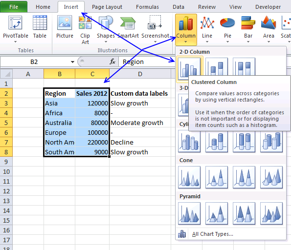
Exclude chart data labels for zero values | MrExcel ... It is a bar chart and I'm trying to figure out how not to display the LABELS for the 0 values. I was using #N/A in my cell formula, which doesn't display a VALUE on the chart. However, when I turn on the LABELS for that data series, there are labels for the 0 values at the bottom of the chart (although there are no bars showing).
Remove data labels from excel chart
How to add data labels from different column in an Excel ... Click any data label to select all data labels, and then click the specified data label to select it only in the chart. 3. Go to the formula bar, type =, select the corresponding cell in the different column, and press the Enter key. See screenshot: 4. Repeat the above 2 - 3 steps to add data labels from the different column for other data points. Change the format of data labels in a chart - Microsoft Support To get there, after adding your data labels, select the data label to format, and then click Chart Elements > Data Labels > More Options. To go to the appropriate area, click one of the four icons ( Fill & Line, Effects, Size & Properties ( Layout & Properties in Outlook or Word), or Label Options) shown here. How to add or remove data labels with a click - Goodly Step 1) Add the Dummy values to the chart Note few things The data labels are turned - ON The 2 products (dummy calculations) are added on the primary axis See this - If you don't know how to add values to the chart Step 2) Place the dummy on the secondary axis Select the 2 data series (one by one) and use CTRL + 1 to open format data series box
Remove data labels from excel chart. Excel Chart delete individual Data Labels First select a data label, which will select all data labels in the series. You should see dark dots selecting each data label. Now select the data label to be deleted. This should remove the selection from all other labels and leave the specific data label with white selection dots. Deletion now will remove just the selected data point. excel - remove data labels automatically for new columns ... I have a query that populates data set for a pivot table. I want data labels to always be at none. Whenever a new column shows up the data label comes back. Anyway I can permanently remove them from the entire pivot chart? this what it looks like when i remove data labels: this what it looks like after refreshing data: How to hide zero data labels in chart in Excel? Sometimes, you may add data labels in chart for making the data value more clearly and directly in Excel. But in some cases, there are zero data labels in the chart, and you may want to hide these zero data labels. Here I will tell you a quick way to hide the zero data labels in Excel at once. Hide zero data labels in chart Change the format of data labels in a chart To get there, after adding your data labels, select the data label to format, and then click Chart Elements > Data Labels > More Options. To go to the appropriate area, click one of the four icons ( Fill & Line, Effects, Size & Properties ( Layout & Properties in Outlook or Word), or Label Options) shown here.
How to Create a Milestone Chart in Excel in 3 Steps ... Steps to Create a Milestone Chart in Excel. I have split the entire process into three steps to make it easy for you to understand. 1. Set Up Data. You can easily set up your data for this chart. Make sure to arrange your data like below data table. How can I hide 0-value data labels in an Excel Chart? How can I hide 0-value data labels in an Excel Chart? Right click on a label and select Format Data Labels. Go to Number and select Custom. Enter #"" as the custom number format. Repeat for the other series labels. Zeros will now format as blank. NOTE This answer is based on Excel 2010, but should work in all versions How to suppress 0 values in an Excel chart | TechRepublic You'll still see the category label in the axis, but Excel won't chart the actual 0. Now, let's use Excel's Replace feature to replace the 0 values in the example data set with the NA ... Excel Pivot Table Report - Clear All, Remove Filters, Select ... 9. Sort Data in a Pivot Table Report - Sort Row & Column Labels, Sort Data in Values Area, Use Custom Lists. 10. Pivot Table Report Layout, Compact, Outline and Tabular Form, Pivot Table Styles and Style Options, Design tab. 11. Pivot Chart Report: Create, Clear and Delete a Pivot Chart report, Pivot Chart Filter Pane, Pivot Chart and Regular ...
Removing datalabels (VBA) - MrExcel Message Board You have to use Points (index) object with it to define which DataLabel you are referring to. Code: Sub t () With Charts ("chart1") With .SeriesCollection (1).Points (2) If .HasDataLabel = True Then .DataLabel.Delete End With End With End Sub I didn't test this, just copied a snipet from the help file and modified it. Excel 2010 Remove Data Labels from a Chart - YouTube How to Remove Data Labels from a Chart Prevent Overlapping Data Labels in Excel Charts - Peltier Tech Overlapping Data Labels. Data labels are terribly tedious to apply to slope charts, since these labels have to be positioned to the left of the first point and to the right of the last point of each series. This means the labels have to be tediously selected one by one, even to apply "standard" alignments. How to remove a legend label without removing the data ... In Excel 2016 it is same, but you need to click twice. - Click the legend to select total legend - Then click on the specific legend which you want to remove. - And then press DELETE. If my reply answers your question then please mark as "Answer", it would help others to find their solution easily from your experience. Thanks Report abuse
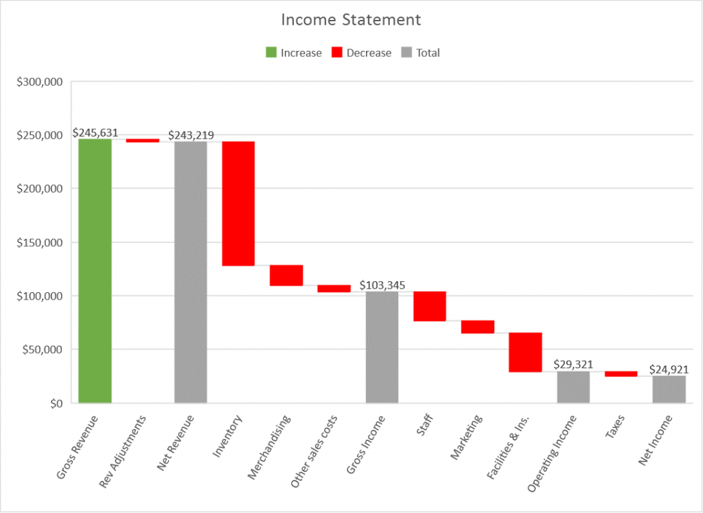
Introducing the Waterfall chart—a deep dive to a more streamlined chart ...
How to Remove Dots from Labels [SOLVED] - Excel Help Forum For a new thread (1st post), scroll to Manage Attachments, otherwise scroll down to GO ADVANCED, click, and then scroll down to MANAGE ATTACHMENTS and click again. Now follow the instructions at the top of that screen. New Notice for experts and gurus:
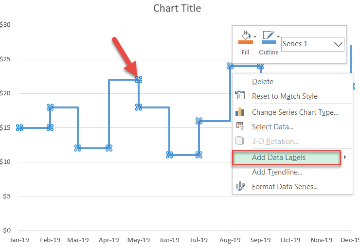
How to Create a Step Chart in Excel - Automate Excel
Adding/Removing Data Labels in Charts - Excel General ... Code ActiveChart.SeriesCollection (2).DataLabels.Select ActiveChart.SeriesCollection (2).Points (8).DataLabel.Select Selection.Delete But other macros in my spreadsheet routinely (and purposefully) alter the chart so that the data point 8 may not always be there (creating a reference error)...
Create Charts in Excel - Easy Excel Tutorial
Edit titles or data labels in a chart - Microsoft Support The first click selects the data labels for the whole data series, and the second click selects the individual data label. Right-click the data label, and then click Format Data Label or Format Data Labels. Click Label Options if it's not selected, and then select the Reset Label Text check box. Top of Page

Enable or Disable Excel Data Labels at the click of a button - How To ...
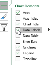
How to add or move data labels in Excel chart? In Excel 2013 or 2016. 1. Click the chart to show the Chart Elements button . 2. Then click the Chart Elements, and check Data Labels, then you can click the arrow to choose an option about the data labels in the sub menu. See screenshot: In Excel 2010 or 2007. 1. click on the chart to show the Layout tab in the Chart Tools group. See ...
Enable or Disable Excel Data Labels at the click of a button - How To ...
Excel tutorial: How to add and remove data series Finally, if you're using Excel 2013 or later, you can also add data series with the chart filter. The trick here is to first include all data, then use the chart filter to remove the series you don't want. For example, here I can select the chart, then drag the data selector to include all 3 tests and the 2 quizzes. I don't want to include the ...
Excel 2010 Remove Data Labels from a Chart - YouTube
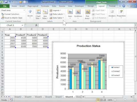
Enable or Disable Excel Data Labels at the click of a ... Select and to go Insert tab > Charts group > Click column charts button > click 2D column chart. This will insert a new chart in the worksheet. Step 2: Having chart selected go to design tab > click add chart element button > hover over data labels > click outside end or whatever you feel fit. This will enable the data labels for the chart.

How to Add Data Labels in Excel - Excelchat | Excelchat
Remove Zero from Chart Data Labels #Shorts - YouTube #ExcelShorts #ExcelChartsHello Friends,In this video, you will learn how to remove zeros form chart data labels.Download our free Excel utility Tool and impr...
Custom data labels in a chart | Get Digital Help - Microsoft Excel resource
Add / Move Data Labels in Charts - Excel & Google Sheets ... Double Click Chart Select Customize under Chart Editor Select Series 4. Check Data Labels 5. Select which Position to move the data labels in comparison to the bars. Final Graph with Google Sheets After moving the dataset to the center, you can see the final graph has the data labels where we want.
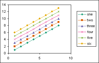
Making a scatter plot in Excel Mac 2011 - YouTube
Add or remove data labels in a chart On the Design tab, in the Chart Layouts group, click Add Chart Element, choose Data Labels, and then click None. Click a data label one time to select all data labels in a data series or two times to select just one data label that you want to delete, and then press DELETE. Right-click a data label, and then click Delete.
How To... Add and Change Chart Titles in Excel 2010 - YouTube
How to add or remove data labels with a click - Goodly Step 1) Add the Dummy values to the chart Note few things The data labels are turned - ON The 2 products (dummy calculations) are added on the primary axis See this - If you don't know how to add values to the chart Step 2) Place the dummy on the secondary axis Select the 2 data series (one by one) and use CTRL + 1 to open format data series box
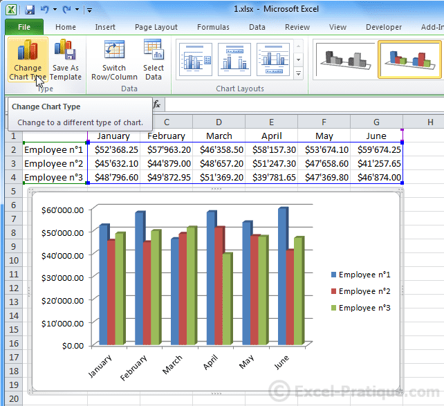
Excel Course: Inserting Graphs
Change the format of data labels in a chart - Microsoft Support To get there, after adding your data labels, select the data label to format, and then click Chart Elements > Data Labels > More Options. To go to the appropriate area, click one of the four icons ( Fill & Line, Effects, Size & Properties ( Layout & Properties in Outlook or Word), or Label Options) shown here.

Chapter 3 Excel 2007/2010 Charts
How to add data labels from different column in an Excel ... Click any data label to select all data labels, and then click the specified data label to select it only in the chart. 3. Go to the formula bar, type =, select the corresponding cell in the different column, and press the Enter key. See screenshot: 4. Repeat the above 2 - 3 steps to add data labels from the different column for other data points.

410 How to display percentage labels in pie chart in Excel 2016 - YouTube
Legends in Excel Charts - Formats, Size, Shape, and Position - Peltier ...
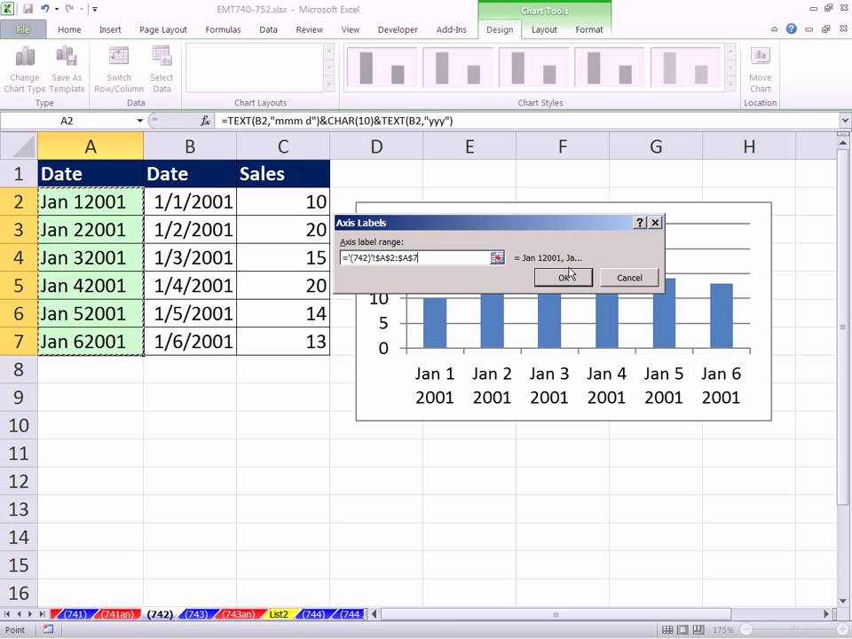
Excel Magic Trick 742: Wrap Text In Chart Label Using CHAR function and ...

How to Add Data Labels in Excel - Excelchat | Excelchat

How to format data labels in excel charts and data elements - YouTube
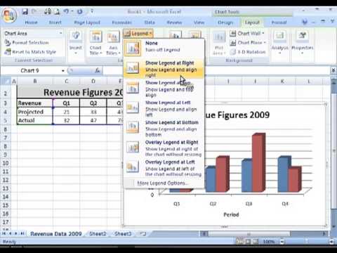
How to add or remove legends, titles or data labels in MS Excel - YouTube
Post a Comment for "42 remove data labels from excel chart"